cnMAE: The Right Metric for Evaluating Solar & Wind Forecasts

With the increasing number of renewable assets comingonline, forecasting is becoming more important for many players within thepower and utility industry. Solar and wind forecasting use high-resolution weather data and AI-powered statistical modeling to predict the amount of energy that will be available at a specific time and location. This way:

·      Independent power producers (IPPs) and energy traders can use short-term solar and wind forecasts to determine how much power to sell into day-ahead markets, and whether to reserve any for real-time markets. This helps them determine whether the market is currently over- orunderpriced when making decisions about mid- and long-term hedging.

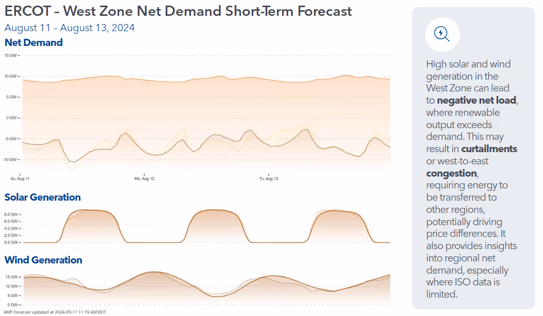
·      Similarly, a growing number of utilities use bottoms-up asset-based forecasts to predict what their net demand will be. These utilities have generation capacity, as well as consumer load, and they need to know in advance how well their assets will perform to avoid buying additional power in expensive, real-time markets.

With these growing use cases, it’s just as important to understand how accurate your forecasts are. The best asset solar and wind forecasts are highly accurate. However, any forecast is going to have a margin of predictive error. “If you’re using asset-level forecasts, it’s important toknow just how accurate they are, because errors can be magnified in yourtrading strategies,” explained Amperon’s Executive Vice President Elliot Chorn. “For instance, if you decide to sell 100 percent of your solar generation, but your forecast is significantly off, you may only sell 90 percent of it. Or worse, you may sell 110 percent.”

The utility industry has several conventional metrics for assessing predictive error in load forecasting. But none of them are the right fit for the unique characteristics of asset forecasting. Amperon proposes the industry standardize around a new metric, cnMAE, to overcome limitations with the following metrics.

MAPE Is Mathematically Unstable

Mean absolute percentage error (MAPE) is perhaps the most common accuracy metric for load forecasting. MAPE is calculated by first subtracting actual load or generation from the predicted amount to determine the size of the difference—or “error.” Then the (absolute) error value is divided by the actual observed amount (or percentage) error. This is calculated for each hour and then averaged over a period of weeks or months to determine MAPE.

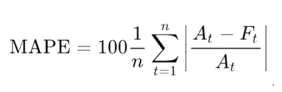
So, for example, a demand forecast may predict electricity consumption of 20 units for tomorrow between 12:00-1:00 pm. If the actual consumption turns out to be 25 units, the first step in calculating MAPE is to determine the absolute difference between the forecast and the actual consumption for that hour. In this instance, it is 5 units. Next, the difference (or error) is stated as a percentage of the predicted amount. Five divided by 25 gives the percentage: 20%. You would then do the same calculation for each hour and average them out to get the MAPE for the period you are evaluating.

MAPE provides a clear measure of load forecasting accuracy that is easy to understand and interpret. Lower MAPE values indicate more accurate forecasts—and by extension, better forecasting models and/or data. However, the calculation can fail when applied to solar generation forecasting.

With asset-level generation, it’s not unusual for actual figures to be zero. In those instances, the standard MAPE calculation would then require dividing the error amount by zero, which is mathematically impossible. Very small figures approaching zero also impair the usefulness of the metric by hyper-inflating the percentage calculation.

nMAE Exaggerates Seasonal Variation

Normalized mean absolute error (nMAE) solves the instability problem that can occur when using MAPE, but it introduces a separate problem for solar forecasts specifically.

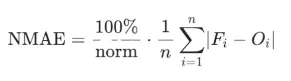
Normalization does away with zero- and near-zero figures before determining the percentage error. Typically, this is done by averaging the actual observed figures from the week or month, before using it to calculate daily error percentages. Normalizing actual generation figures keeps them from approaching zero and throwing off the metric.

However, nMAE doesn’t account for seasonal variations in solar output capacity. So, in the winter, when average solar generation is minimal, it often exaggerates forecast errors, and when generation is at its highest in the summer, nMAE can underestimate errors. Consider, for example, a winter forecast that is for two units of solar production, but only one actual unit (on average) is generated. The error would be 1 unit, and the nMAE would be 100%. Now consider a summer forecast that is for 11 units of solar production, but only 10 units are produced (on average). The error is the same: 1 unit. But now the nMAE would be only 10%.

nMAE is good for comparing forecasting models that deal with different types of data. It is acceptable for wind forecasts, too, as wind generation is less subject to seasonal variation. But it requires further normalization to make it a useful benchmark for seasonally-dependent solar forecasting.

RMSE Isn’t Relative to Size

Root Mean Squared Error (RMSE) is another common forecasting metric with only limited usefulness in solar and wind forecasting.

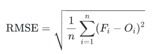
Like the metrics above, RMSE is calculated by first determining the difference between predicted amounts and the actual observed amounts for a given period. For RMSE, each difference is then squared to remove negative values and to give greater weight to larger errors. Next, the squared differences are averaged, and the final step is to take the square root, which returns the value to the original unit-scale of the data.

RMSE, like nMAE, overcomes the mathematical instability of dividing by zero or near-zero values. RMSE is more consistent than nMAE across seasonal variations in solar capacity; however, it is sensitive to scale. Because RMSE is stated in the original units of measurement, it doesn’t account for the size of the solar or wind installation or the average yield from that asset over the period we’re examining.

For example, the RMSE of 250 kilowatts (kW) for a 20 megawatt (MW) wind farm would be an order of magnitude more accurate than the same RMSE for a 2MW wind farm. But because the relative size of the installation is not represented in the metric, RMSE is inappropriate for comparing forecasts across a range of installation sizes.

cnMAE: The Goldilocks Metric

After considering numerous metrics, including many proposed at Solar Forecast Arbiter, Amperon concluded that the most useful measurement of predictive error for asset renewables forecasting is nMAE with an additional normalization step forcapacity: cnMAE, or capacity-normalized mean absolute error.

“cnMAE doesn’t have the shortcomings that MAPE and nMAE have for market participants that need to rely on solar forecasting,” Chorn said. “Plus, it’s a more valuable tool than RMSE for power producers that want to make decisions based on comparisons of assets within a varied portfolio of wind and solar installations.”

The benefits of cnMAE make it the just-right metric for solar and wind forecasting:

·      Prevents Unintended Bias: Unlike other measurements, cnMAE maintains an unbiased context by providing capacity-normalized insights and reducing sensitivity to seasonality.

·      Supports Comparability: cnMAE enables performance comparison between systems with different capacities. This makes it an ideal metric for diversified portfolios of single-site installations.

·      Enhances Planning and Budgeting: Power producers can better prioritize maintenance and operations with the capacity-adjusted insights of cnMAE.

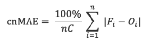
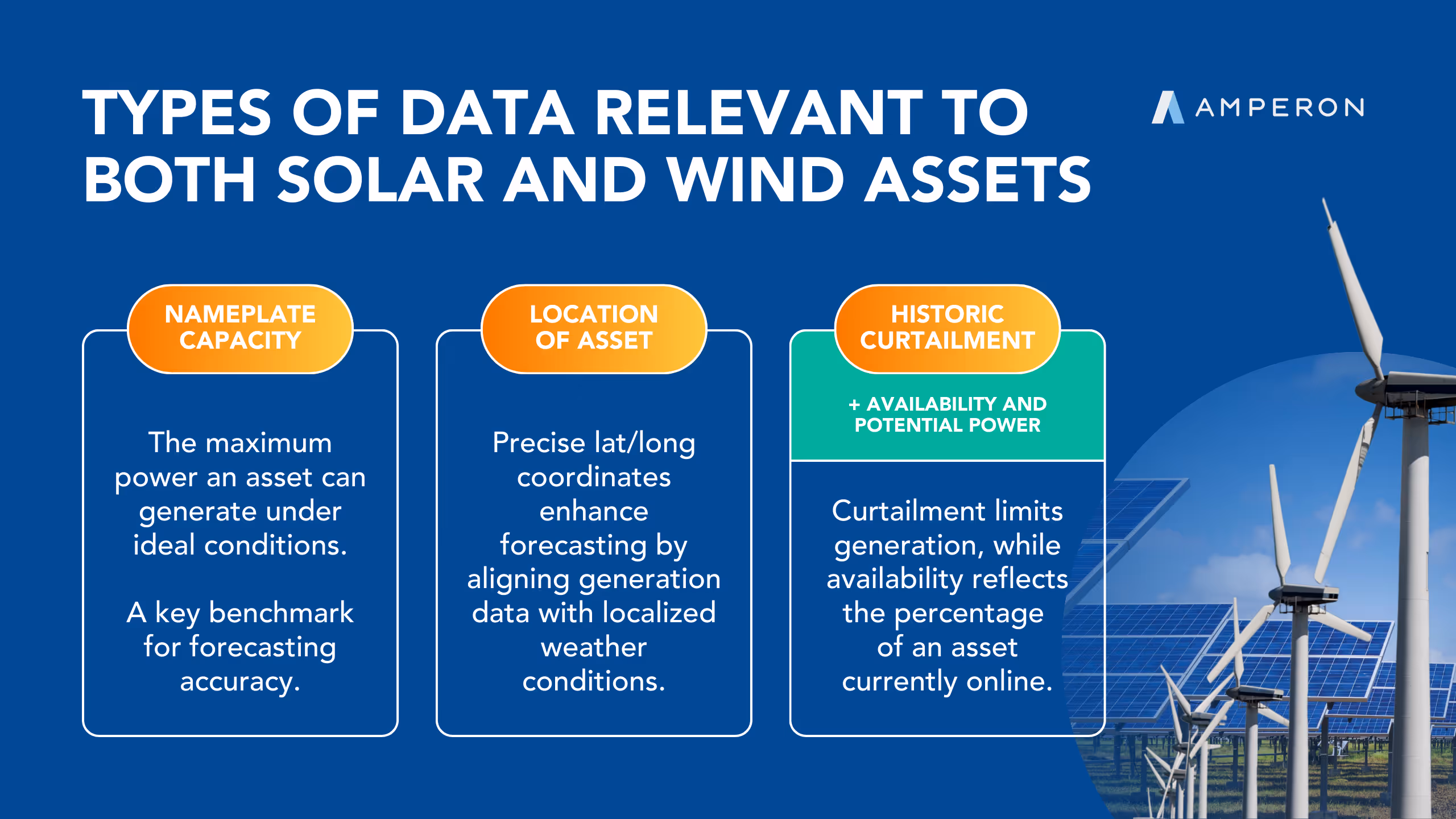
cnMAE normalizes for capacity by scaling the forecast errorrelative to a anasset’s rated nameplate capacity. Simply put, cnMAE = MAE / Capacity.

cnMAE in the Context of a Day

In addition to conventional forecasting metrics, Amperon provides its asset forecasting clients with cnMAE, which has consistently proven more useful. Take for example, a 20MW solar installation owned by one of our Midwestern IPP clients. The table below shows the actual hourly generation for a day in April, followed by the forecasted generation, the absolute error, the MAPE, and the cnMAE.

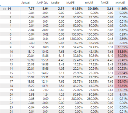
For the hour ending (HE) at 1 a.m. in the middle of the night, the prediction was spot on—no solar output. For the next hour, still in the middle of the night, the absolute error was miniscule: 0.01. But due to its mathematical instability, the MAPE is 50%. By comparison, the normalized cnMA Eis a mere 0.08% and better reflects the insignificance of the error. The instability is much more noticeable at 7 a.m., when the sun is just beginning to come up. The forecast predicted a small amount of generation (0.44 MW), but there was none. In fact, demand can be negative at night when the photovoltaic inverters consume electricity. cnMAE shows the error as 2.39%. But because MAPE divides the predicted amount by the near-zero actual (-0.04), it calculates an enormous MAPE of 1,200%.

Over the course of the day, the absolute errors range from 0.0 to a high of 7.68. cnMAE tracks closely to the ups and downs in absolute error, ranging from 0.0% to a high of 38.4%. By comparison, MAPE ranges from 0.0% to 1,200% and does not correlate to the ups and downs of the absolute errors over the course of the day. The correlation and moderate range of cnMAE is radically more useful as an hour-to-hour measurement, and as a result, the average cnMAE for the day (11.86%) is inherently more accurate than the average MAPE (91.55%).

cnMAE in Seasonal Context

The advantages of cnMAE over nMAE are particularly obvious when looking at examples from two different times of the year. Table 2 shows averages for the same solar installation for the month of January and the month of April.

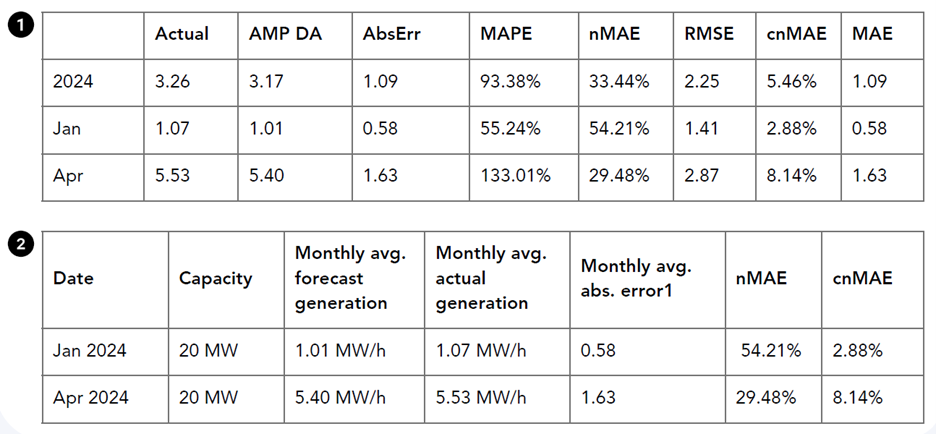
For January, when solar radiation is typically low in the northern hemisphere, the average hourly forecast was for 1.01 MW of generation. This was very close to the actual average hourly generation of 1.07 MW. The monthly average of hourly absolute errors was 0.58, which is a small figure, but nonetheless produces a significant nMAE (54.21%) when divided by the low actual generation figure.

In April, the monthly average hourly absolute error was roughly three times greater (1.63) than in January, but because the actual generation figure was so much larger in April (5.53 MW/h) the nMAE score was minimized (29.48%).

By comparison, the cnMAE score normalizes these error figures against the capacity of the installation (20 MW) instead of the actual generation figure. Relative to the large size of the solar farm, the forecasting error in January is quite small, and this is reflected in the cnMAEscore (2.88%). The April forecasting error was larger than the January error, and again, the cnMAE score (8.14%) reflects this.

cnMAE in Site Comparison

cnMAE also proves more useful than RMSE when comparing the accuracy of forecasts between solar installations of different sizes. Table 3 shows figures for the 20 MW solar farm from the examples above. Table 4 shows figures for a smaller installation, owned by the same IPP, that has a capacity of only 1.75MW.

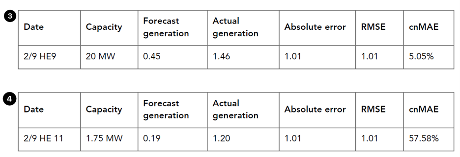
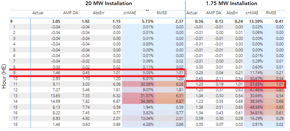
Note that the absolute error is the same but on different hours for the two different solar farms. Relative to capacity of the 20 MW installation, the error is rather small, whereas it represents a much greater proportion of the potential capacity of the 1.75 MW installation. The RMSE score, which is the same in both tables, doesn’t reflect this perspective at all. cnMAE does, however, making it a useful metric for making comparisons and prioritizations within a portfolio.

In Conclusion

Predictive error, though inevitable, can have a profound impact on decision making and outcomes that rely on forecasting in the utility industry. Solar and wind forecasting will continue to grow in importance for the operations of utilities and IPPs, as well as for the speculative decisions of energy traders. To accelerate the maturity of renewable asset forecasting in the market, Amperon believes the industry should coalesce around a single, well-suited measure of predictive error. In our experience, cnMAE is the best option.